How Neural Networks Work: The Mathematics of Machine Intuition

For over half a century, computing was bound by a rigid, unyielding philosophy: if a human could not explicitly formulate the exact rule, a computer could not perform the task.

If you wanted a machine to recognize a handwritten number "8", you had to author hundreds of lines of fragile conditional logic: Check if there is a top loop; test if the bottom loop is circular; confirm the waist pinches in the center. But as soon as someone scribbled an italicized, tilted, or imperfect "8", the rigid rules shattered. The real physical world is messy, noisy, and infinitely diverse—qualities that traditional software was never built to navigate.

In the 1940s and 50s, visionary researchers asked an audacious question: What if, instead of programming computers with rules, we designed systems that learn from examples just like the human brain?

The answer is the Artificial Neural Network (ANN). Today, neural networks power the voice recognition in your phone, guide autonomous vehicles through rainy nighttime traffic, predict the complex 3D folds of life-saving proteins in seconds, and generate human-level prose and code.

Yet beneath all the mystique of "artificial intelligence," a neural network is not magic. It is an awe-inspiring, harmonious symphony of linear algebra, calculus, and probability.

Anatomy of an Artificial Neuron: The Perceptron

To understand a deep network with hundreds of billions of connections, we must first examine its fundamental building block: the single artificial neuron, historically termed the Perceptron.

In biological neurobiology, a brain cell receives electrical chemical impulses through branching structures called dendrites. If the combined electrical potential inside the cell body (the soma) crosses a critical threshold, the neuron fires an action potential down its axon to stimulate adjacent cells.

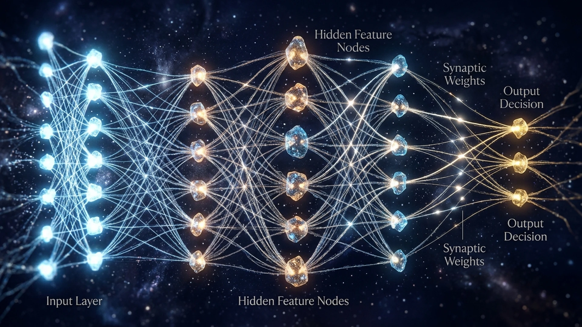
An artificial neuron mirrors this biological machinery using pure mathematics:

1. Inputs ($x_1, x_2, \dots, x_n$): These are numbers fed into the neuron. For a computer vision system, each input might be the grayscale brightness value of a single pixel (ranging from $0.0$ for pitch black to $1.0$ for pure white).
2. Synaptic Weights ($w_1, w_2, \dots, w_n$): Every input connection possesses a unique "weight"—a real number that dictates how much influence that specific input has on the neuron's decision. A high positive weight amplifies the signal; a negative weight acts as an inhibitor.
3. The Bias ($b$): A single adjustable offset added to the sum, representing how easily the neuron gets triggered regardless of the incoming inputs.
4. Weighted Sum ($z$): The neuron multiplies every input by its corresponding weight and adds the bias: $$z = \sum_{i=1}^{n} (w_i \cdot x_i) + b = w_1 x_1 + w_2 x_2 + \dots + w_n x_n + b$$
5. The Activation Function ($\sigma$ or $f$): Finally, the weighted sum passes through a mathematical function that introduces non-linearity and determines the neuron’s final output signal ($a = f(z)$).

Scientific Diagram of Neural Network Forward Propagation and Synaptic Weights

The Non-Linear Superpower: Why Activation Functions Matter

Why can’t we just pass the linear sum $z$ directly to the next neuron?

In mathematics, if you multiply a linear equation by another linear equation, the resulting combination is still strictly linear. If an entire 100-layer neural network used only linear operations, the entire multi-billion dollar architecture would collapse into nothing more than a single high-school linear equation: $y = mx + b$.

A purely linear system can only draw straight dividing lines through data. It could never solve the classic XOR (exclusive OR) problem, separate intertwined spirals, or recognize a human face smiling versus frowning.

Activation functions provide the non-linear "elbow grease" that allows neural networks to approximate virtually any mathematical curve or surface:

• ReLU (Rectified Linear Unit): Defined simply as $f(z) = \max(0, z)$. If the input is negative, the neuron stays silent ($0$); if positive, the signal passes through directly. ReLU is the workhorse of modern deep learning because it calculates at blinding speed on GPUs and avoids the vanishing gradient problem.
• Sigmoid: Curves the input into an S-shaped smooth probability between $0.0$ and $1.0$: $\sigma(z) = \frac{1}{1 + e^{-z}}$. Often used in binary decision outputs.
• Softmax: Applied at the final output layer of a multi-class network, converting raw output numbers into a normalized probability distribution that sums cleanly to $100%$.

Forward Propagation: The Cascading Waves of Thought

A modern deep neural network arranges artificial neurons into distinct, interconnected layers:

1. Input Layer: Receives the raw sensory data (e.g., a $28 \times 28$ image of a handwritten digit, totaling $784$ input neurons).
2. Hidden Layers: The intermediate tiers between input and output. The term "deep learning" simply refers to networks with many stacked hidden layers. Early hidden layers learn simple primitives—detecting horizontal edges, vertical boundaries, and diagonal corners. Intermediate hidden layers combine these edges into shapes: loops, circles, intersections. Deepest hidden layers assemble shapes into high-level conceptual features: noses, eyes, wing feathers, or digits.
3. Output Layer: Yields the final verdict. For digit recognition, it contains 10 neurons (representing numbers $0$ through $9$). The neuron with the highest firing activation represents the network's prediction.

During Forward Propagation, data cascades from left to right. Matrices of weights multiply vectors of activations, biases are added, activation functions fire, and within milliseconds, raw pixels become an informed hypothesis: "I am 98.7% confident this photo is an 8."

How Machines Learn: Backpropagation & Gradient Descent

When a newly initialized neural network is born, its synaptic weights are assigned completely random numbers. If you show it a photo of a handwritten "8", its initial guess will be hopelessly wrong: "I think this is a toaster with 92% confidence."

How does a collection of dumb numbers transform itself into an expert classifier?

Step 1: The Loss Function (Measuring the Blunder)

First, the network needs a mathematical mirror to assess how far off it was. The Loss Function computes a scalar number representing the error between the network's output prediction ($\hat{y}$) and the true ground-truth label ($y$). If the error is large, the loss is high; if the network guesses perfectly, the loss sinks to zero.

Step 2: The Error Gradient Landscape

Imagine you are standing blindfolded on a foggy, mountainous terrain in the middle of the night, and your goal is to find the lowest valley floor (the point of minimum loss). Although you cannot see the landscape, you can feel the slope of the ground beneath your boots with your walking stick.

The steepness and direction of that slope is the Gradient ($\nabla L$). It is a vector of partial derivatives calculated using the chain rule of calculus: $$\frac{\partial L}{\partial w_{ij}} = \frac{\partial L}{\partial a_k} \cdot \frac{\partial a_k}{\partial z_k} \cdot \frac{\partial z_k}{\partial w_{ij}}$$

Step 3: Backpropagation (Nudging the Synapses)

Invented in foundational forms by researchers including David Rumelhart, Geoffrey Hinton, and Ronald Williams in 1986, Backpropagation calculates the gradient of the loss with respect to every single weight in the network, moving systematically backward from the output layer to the input layer.

Once the slopes are known, Gradient Descent updates each weight by taking a small step in the opposite direction of the gradient: $$w_{\text{new}} = w_{\text{old}} - \eta \cdot \frac{\partial L}{\partial w}$$

The parameter $\eta$ (Greek letter eta) is the Learning Rate. If $\eta$ is too high, the updates leap over the valley and tumble down the cliff; if $\eta$ is too low, learning crawls like molasses.

By repeating this dance—feeding millions of examples forward, measuring the error, and rippling the corrections backward—the network automatically tunes billions of weights until its accuracy approaches near perfection.

Fast Facts About Neural Networks

• The Mark I Perceptron (1958): The world's first hardware neural network, built by Frank Rosenblatt, was a custom vacuum-tube mainframe weighing over five tons, connected by a sprawling tangle of physical potentiometer cables adjusted by electric motors!
• Universal Approximation Theorem: Mathematicians proved that even a single hidden layer with a sufficient number of non-linear neurons can approximate any continuous mathematical function to arbitrary precision.
• The Scale of Modern AI: Frontier models such as GPT-4 and Claude 3 contain hundreds of billions—and in some architectures, trillions—of parameters, requiring clusters of tens of thousands of specialized Tensor Processing Units (TPUs) or GPUs operating in parallel.
• AlphaFold's Biological Miracle: By training deep attention neural networks on known protein geometries, DeepMind's AlphaFold solved the 50-year-old grand challenge of biology, predicting the 3D structures of over 200 million cataloged proteins in nature.

Whether sorting recycled plastics, translating ancient languages, or decoding gravitational waves from black hole collisions, neural networks represent humanity's greatest triumph in teaching machines how to perceive, learn, and reason.